Vineyard going green or turning yellow?
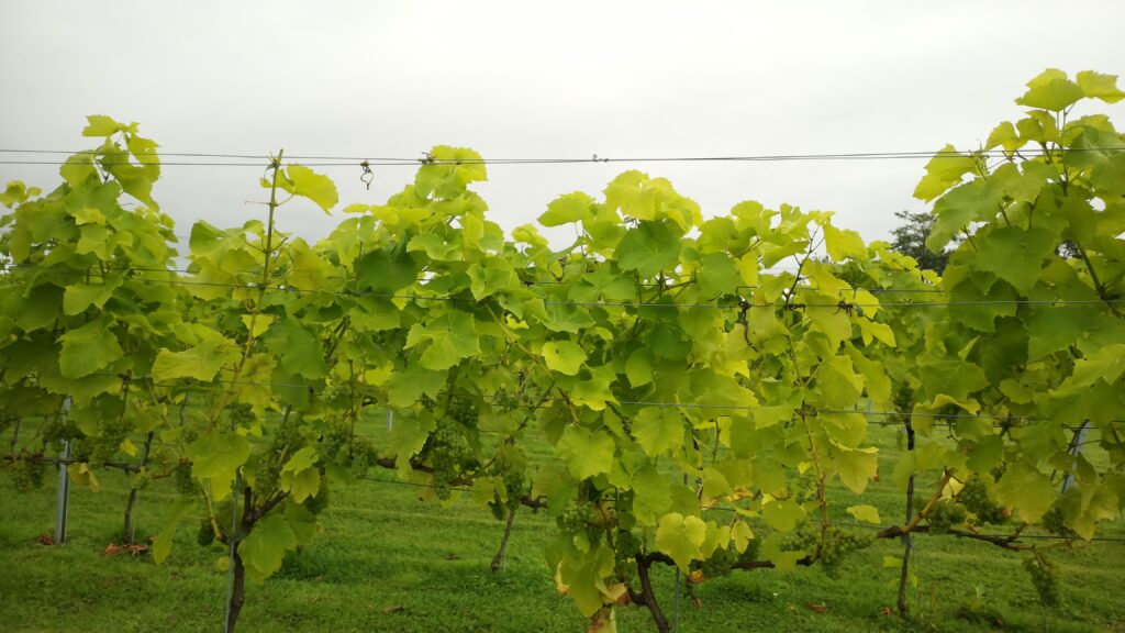
about contact Vineyard managers can’t change the amount of sun or rain that their vines receive but they can ensure that vines extract the maximum amount of energy from the available sun’s rays. Latest results from the South Wales Llanerch Vineyard trial demonstrate how to accurately measure the leaf pigments and rapidly determine when to […]
Drones in the vineyard
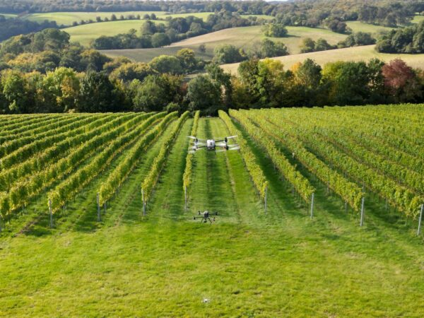
about contact Drones at JoJo’s vineyard, Russell’s Water Oxfordshire UAVs have long been discussed as a way to survey vineyards for vine health and apply directed nutrition or phytosanitary interventions. Great in theory but impractical? A few days ago Corbeau saw a demonstration of the new DJI AGRAS T50 at JoJo’s vineyard just outside Henley-upon-Thames […]
Smartphone spectral leaf imaging
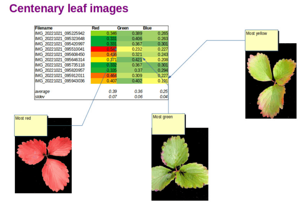
about contact Strawberry leaf images and Red Green Blue indices derived using OpenCV image analysis All season we have been monitoring the health of our Strawberry Greenhouse crop. In addition to visual inspection with a loupe, digital leaf imaging has been a useful way to follow the development of the plants. Now that autumn has […]
Mineral deficiency in bean leaves classified by multispectral imaging
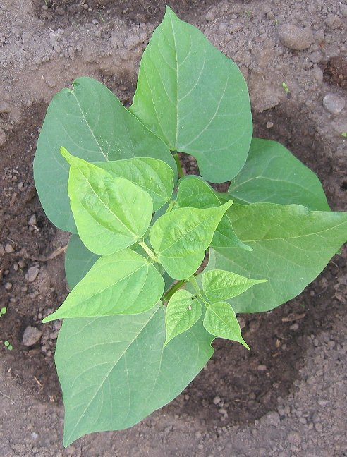
about contact French bean plant Plants tell us when they are lacking vital nutrients but we can’t always hear what they are saying. Nitrogen, phosphorous and potassium (N, P, K) are well know macronutrients and the appearance of plants lacking any one of them is also well known. Plants lacking nitrogen have small leaves and […]
Coffee leaf miner infection located by multispectral imaging
about contact news There’s an awful lot of coffee in Brazil! according to the old song recorded by Frank Sinatra. In 2021 almost 70 million 60kg bags of coffee were produced in Brazil, roughly one third of global production, making Brazil the largest coffee producer in the world. Yield varies from year to year depending […]
Raman spectroscopy sorts male hemp plants from females
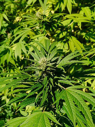
about contact news Cannabis sativa (courtesy Wikipedia) It turns out that growers of medicinal cannabis and those catering for a more recreational market love females but hate males. Gender bias is certainly in the news today but horticulturalists have long known that female hemp plants have higher levels of pharmacologically active compounds than male plants. […]
Precision viticulture coming to fruition
Mists, check. Mellow fruitfulness, check. Maturing sun, – eventually check! In the UK the 2021 growing season has been good but not exceptional. A late spring followed by a warm June and July gave way to a disappointing August with plenty of warm damp days to encourage the development of mildew. It has been fascinating […]
Cassava virus infection detected with handheld multispectral imager
One of the most important sources of carbohydrate energy in equatorial countries comes from the cassava plant. It looks like a trendy house plant but the roots are large tubers that provide valuable nutrition. Tubers can be boiled and mashed or dried, ground and turned into flour. Cassava is a robust crop but suffers from […]
Counting grapes with machine learning
As the grapes swell in the late summer sun and rain, vignerons start thinking about the harvest. What is the yield going to be? how much sugar will there be in the grapes and finally how many bottles of wine can be made? It would be really useful to have a way to predict the […]
Smarts or knowledge – which one wins at precision agriculture?
Imagine a competition to produce the highest yields of winter wheat between Sheldon Cooper and a winner of the Apprentice. Who would win? It’s tempting to choose the Big Bang brain-box but what if Lord Sugar’s apprentice had spent 10 years working on arable farms in the UK, Australia and the USA before joining the […]